IMCD estimator examples

library(AIDA)

This vignette reproduces the examples presented in Loureiro et al. (2026). The real-life examples included here are the Cars and Spotify Tracks datasets, which are discussed in Sections 6.1 and 6.2 of the paper, respectively. The datasets are available in the package and can be loaded using data("intCars") and data("spotify_tracks").

The intData class is used to create objects that represent interval-valued data. The IMCD function computes the reweighted IMCD estimates, which are robust estimates of location and scatter for interval-valued data. The function allows for different cutoff methods and levels for a one-step reweighting process. The function int_outliers identifies potential outliers in interval-valued data using robust distance-based methods with customizable cutoff criteria. The examples provided here demonstrate how to apply these methods to real datasets, and the results can be compared to those presented in the paper for validation.

For more details and examples on the intData class, please see the vignette: Class intData examples.

Cars Dataset

This dataset contains interval data of car specifications (Duarte Silva and Brito (2025)), including min-max values. The aggregation of the microdata was done by car model, resulting in $n=27$ observations. It is composed of $5$ variables:

Engine Capacity (EngCap)
Top Speed
Acceleration
Price (lnPrice after log transformation)
Class (values: Berlina, Luxury, Sportive, and Utilitarian)

As no microdata are available, and following the standard assumption in the literature, we adopt a continuous uniform distribution for the latent variables, corresponding to the symmetric and i.d. case with $\delta = 1/12$ . This is the default setting for the intData class.

data(intCars)
cars_microdata <- intCars$microdata
cars_int <- intCars$intData

The IMCD function is used to compute the reweighted IMCD estimates and the robust squared Interval-Mahalanobis distances of each observation from the estimated barycenter. The subset size is set to $\lfloor 0.75\times 27\rfloor=20$ , and the reweighting cutoff to “farness” with a cutoff level of $0.9$ . The int_outliers function identifies potential outliers based on the robust distances obtained from the IMCD estimates, using the same cutoff criteria.

cars_IMCD <- IMCD(cars_int, m = floor(0.75*cars_int@NObs), cutoff = "farness", cutoff_lvl = 0.9)
cars_outliers <- int_outliers(cars_IMCD$robust_dist, cutoff = "farness", cutoff_lvl = 0.9)
cars_outliers$outliers_names
#> [1] "Ferrari"         "HondaNSK"        "MercedesSL"      "MercedesClasseS"
#> [5] "Porsche"

Pairs plot, the lower triangular shows scatter plots of the four variables, with the outlying observations highlighted in red, while the upper triangular shows the interval correlation matrix.

cars_outliers_colors <- rep('gray50', cars_int@NObs)
names(cars_outliers_colors) <- rownames(cars_int)
cars_outliers_colors[cars_outliers$outliers_names] <- 'red'

SYMB.pairs.panels(cars_int, palette = cars_outliers_colors, type = "rectangles", 
                    corr = cov2cor(cars_IMCD$cov_IMCD), labels = colnames(cars_int),
                    is_outlier = cars_outliers$is_outlier, gap = 0)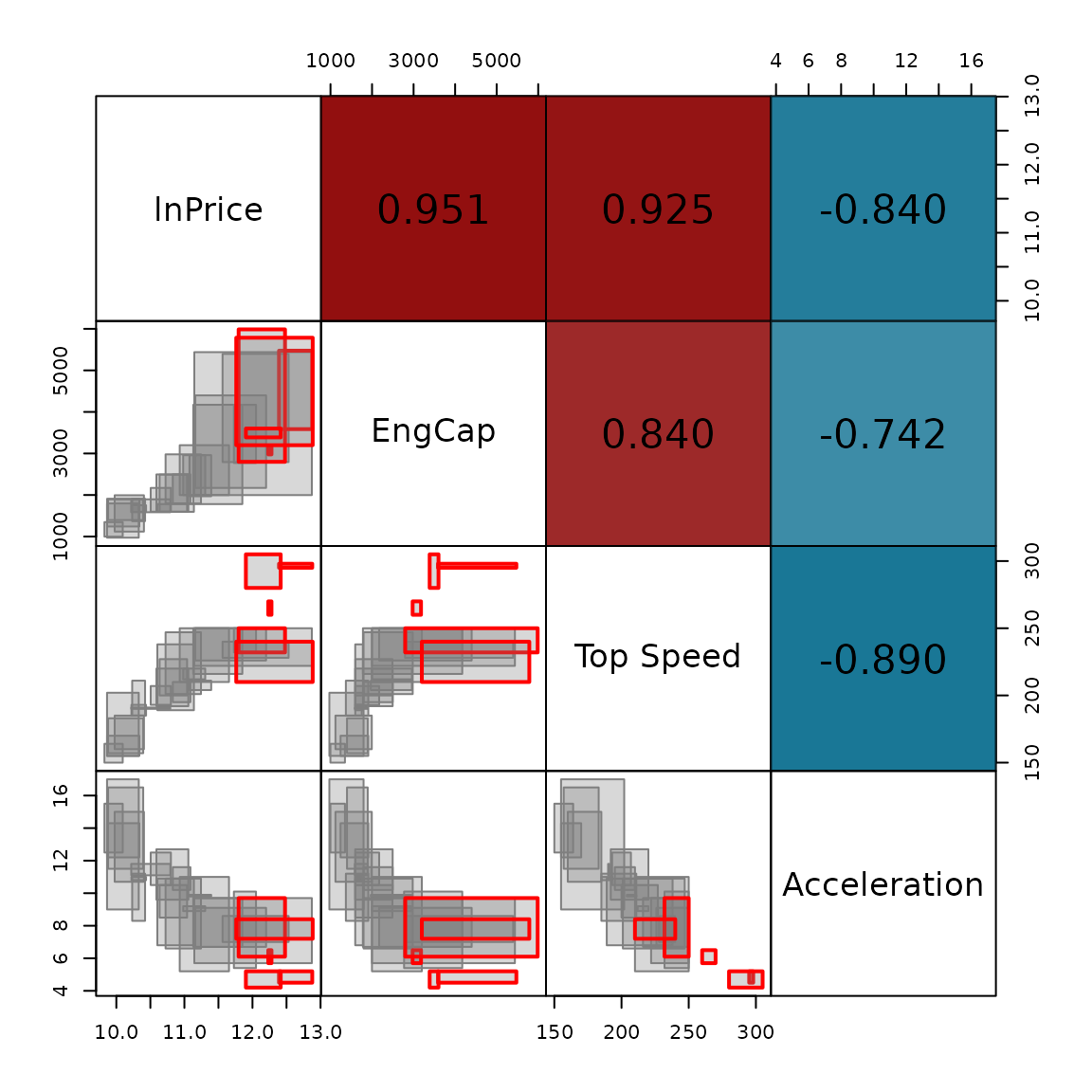

Distance-distance plot of the classical versus robust squared Interval-Mahalanobis distances. The points’ shape represents the car model class, the horizontal and vertical lines correspond to the 0.9 farness cutoff value and the 1.5 adjusted boxplot cutoff value, respectively, with the outliers marked in red.

# Classical distances and outliers
cars_class_dist <- IMah_dist(cars_int, z = rep(1,cars_int@NObs))
cars_class_outliers <- int_outliers(cars_class_dist, cutoff = "adjbox", cutoff_lvl = 1.5)

cars_is_outliers <- as.character(cars_outliers$is_outlier)
cars_is_outliers[cars_outliers$is_outlier] <- "Outlier"
cars_is_outliers[!cars_outliers$is_outlier] <- "Inlier"

plot_dist_dist(cars_class_dist, cars_class_outliers$cutoff_value[[2]], class_cutoff_label = "1.5 Adjbox",
                cars_IMCD$robust_dist, cars_outliers$cutoff_value, rob_cutoff_label = "0.9 Farness",
                color_class = cars_is_outliers, ggplotly = FALSE, shape_class = cars_microdata$class, 
                shape_label = "Class", palette = c("gray50","red"), 
                label_obs = c(cars_outliers$outliers_names, "Bmwserie7"))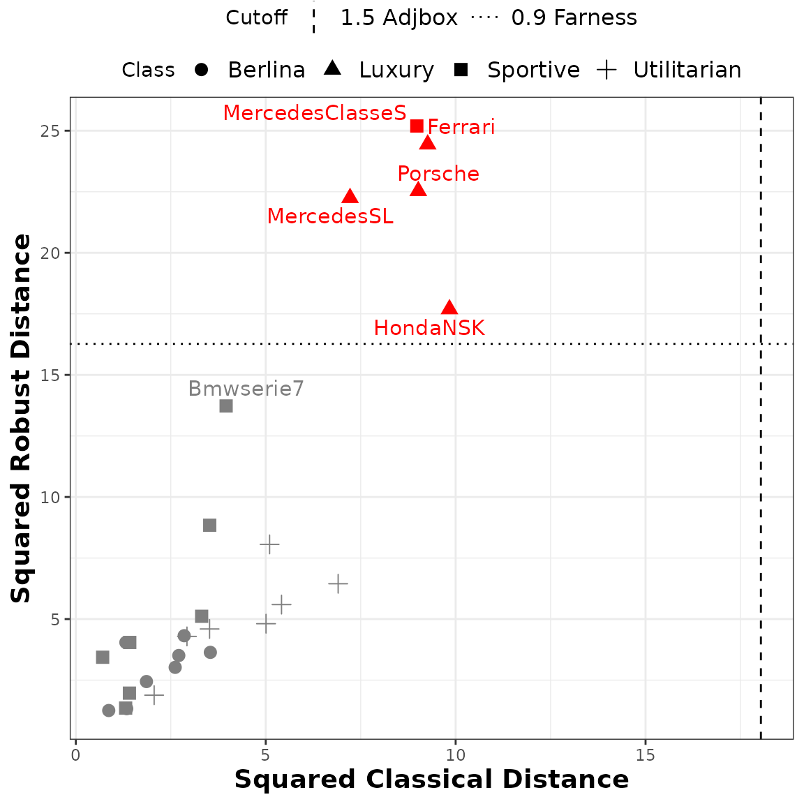

Spotify Tracks Dataset

This dataset contains interval data of Spotify tracks’ audio features (Pandya (2022)), including min-max values and trimmed intervals, as well as the microdata. The aggregation of the microdata was done by track genre, resulting in $n=111$ observations. It is composed of 11 audio features:

duration
danceability
energy
loudness
speechiness
acousticness
instrumentalness
liveness
valence
tempo
popularity

Prior to aggregation, logarithmic transformations were applied to loudness and tempo, duration_ms in milliseconds was converted to duration in minutes, and popularity was scaled to the range $[0,1]$ . The latent variables’ parameters are estimated from the microdata, using Kernel Density Estimation (KDE) (package kde1d). Here, we will use the data aggregated into trimmed intervals, taking as lower and upper bounds the $1\%$ and $99\%$ quantiles, respectively.

data(spotify_tracks)
spotify_int <- spotify_tracks$intData_trimmed

The IMCD estimates are computed using the IMCD function with a subset size of $\lfloor 0.75\times 111\rfloor=83$ , and a reweighting cutoff based on “farness” with a cutoff level of $0.95$ . The int_outliers function applies the outlier detection rule using a “farness” cutoff of $0.95$ to identify strong outliers and $0.9$ for mild outliers.

spotify_IMCD <- IMCD(spotify_int, m = round(0.75*nrow(spotify_int)), 
                      cutoff = "farness", cutoff_lvl = 0.95)

# Strong outliers
spotify_outliers <- int_outliers(spotify_IMCD$robust_dist, cutoff = "farness", cutoff_lvl = 0.95)
spotify_outliers$outliers_names
#> [1] "classical" "comedy"    "grindcore" "sleep"

# Mild outliers
spotify_outliers_2 <- int_outliers(spotify_IMCD$robust_dist, cutoff = "farness", cutoff_lvl = 0.9)
spotify_outliers_2$outliers_names[!spotify_outliers_2$outliers_names%in%spotify_outliers$outliers_names]
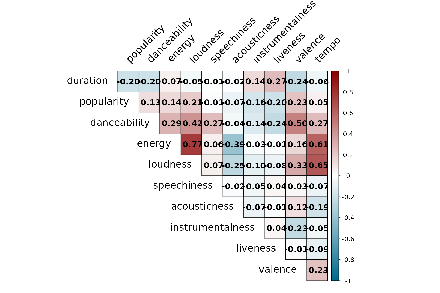
#> [1] "ambient"       "chicago-house" "death-metal"   "iranian"

Interval correlation matrix plot based on the IMCD estimates.

# Compute correlation matrix from the robust covariance matrix
spotify_corr <- cov2cor(spotify_IMCD$cov_IMCD)

colfunc <- colorRampPalette(c("deepskyblue4", "white", "red4"))
corrplot::corrplot(
  spotify_corr,
  method = "color",
  type = "upper",
  diag = FALSE,
  col = colfunc(200),
  tl.col = "black",
  tl.srt = 45,
  tl.offset = 1,
  tl.cex = 1.2,
  outline = TRUE,
  addCoef.col = "black",
  number.cex = 1
)

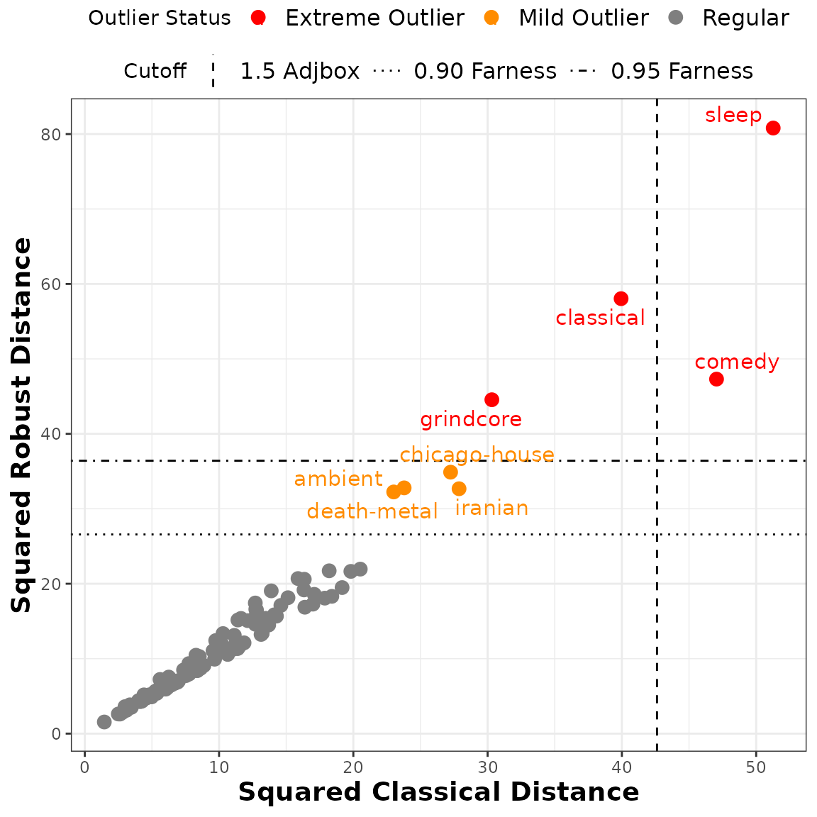
Distance-distance plot of the classical versus robust squared Interval-Mahalanobis distances for the Spotify dataset. The horizontal lines correspond to the $0.9$ and $0.95$ farness cutoff values, with the extreme outliers marked in red and the mild outliers in orange, while the vertical line represents the $1.5$ adjusted boxplot cutoff.

# Classical distances and outliers
spotify_class_dist <- IMah_dist(spotify_int, z = rep(1,spotify_int@NObs))
spotify_class_outliers <- int_outliers(spotify_class_dist, cutoff = "adjbox")

spotify_is_outliers <- as.character(spotify_outliers$is_outlier)
spotify_is_outliers[!spotify_outliers_2$is_outlier] <- "Regular"
spotify_is_outliers[spotify_outliers_2$is_outlier] <- "Mild Outlier"
spotify_is_outliers[spotify_outliers$is_outlier] <- "Extreme Outlier"
palette_outliers <- c(
  "Regular"         = "gray50",
  "Mild Outlier"    = "darkorange",
  "Extreme Outlier" = "red"
)

plot_dist_dist(spotify_class_dist, spotify_class_outliers$cutoff_value[[2]], 
                "1.5 Adjbox", spotify_IMCD$robust_dist, 
                c(spotify_outliers_2$cutoff_value, spotify_outliers$cutoff_value), 
                c("0.90 Farness", "0.95 Farness"), color_class = spotify_is_outliers, 
                color_label = "Outlier Status", palette = palette_outliers, ggplotly = FALSE, 
                label_obs = spotify_outliers_2$outliers_names)

References

Duarte Silva, Pedro, and Paula Brito. 2025. MAINT.Data: Model and Analyse Interval Data. https://doi.org/10.32614/CRAN.package.MAINT.Data.

Loureiro, Catarina P., M. Rosário Oliveira, Paula Brito, and Lina Oliveira. 2026. Minimum Covariance Determinant Estimator and Outlier Detection for Interval-valued Data. https://arxiv.org/abs/2604.26769.

Pandya, Maharshi. 2022. Spotify Tracks Dataset. https://doi.org/10.34740/KAGGLE/DSV/4372070.

Catarina P. Loureiro

Cars Dataset

Spotify Tracks Dataset

References